Multi-Layer Perceptron

This guide will help you build a 3 layer Neural Network from scratch i.e without the use of any existing python libraries.

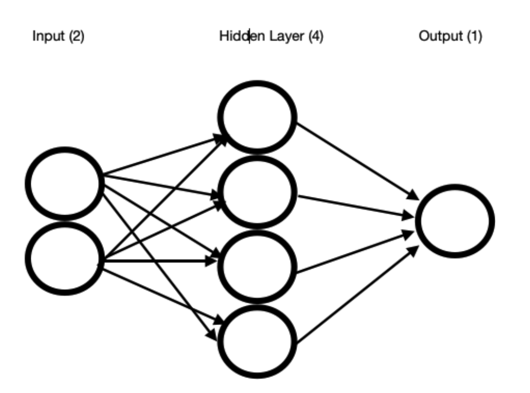
A Neural Network generally takes the form:

Input Layer
Hidden Layer(s)
Output Layer

For this tutorial we will implement a 3 layer NN with 2-\(n_h\)-1 architecture where \(n_h\) stands for the number of hidden nodes.

Some specifications:

Activation function used: Sigmoid
Learning Rate: 0.005
Number of hidden nodes, \(n_h\) = 2,4,6,8,10
Error: Mean Squared Error

Step 1: Load the given train and test datasets.

Step 2: Feature normalize your train and test datasets:

For each feature \(x_i\) , your normalized feature \(y_i\) will be:

yi = (xi - mi)/si      

where \(m_i\) is the mean and \(s_i\) is the standard deviation of the given feature.

Use the same \(m_i\) and \(s_i\) values to normalize your test dataset. Remember, you only transform your test dataset with these values and not fit it using its own mi and si values.

Step 3: Split the train dataset into train and validation sets (an 80/20 split should work)

Step 4: The Multi Layer Perceptron Class and functions:

Our sigmoid activation function and it’s derivatives are defined as follows:

def sigmoid(t):
    return 1/(1+np.exp(-t))
def sigmoid_derivative(g):
    return g * (1 - g)

Our Multi-Layer Perceptron Class is defined as follows:

class MultiLayerPerceptron:
    def __init__(self, x, y,nh):
        self.input      = x
        #random weight initialization
        self.weights1   = np.random.rand(self.input.shape[1],nh) 
        #random weight initialization
        self.weights2   = np.random.rand(nh,1)
        self.y          = y
        self.output     = np.zeros(self.y.shape)
        
    def feedforward(self):
        self.layer1 = sigmoid(np.dot(self.input, self.weights1))
        self.output = sigmoid(np.dot(self.layer1, self.weights2))
        return self.output

    def backpropagation(self):
        '''
        This function calculates new weight vectors and updates 
        the weight for both input 
        to hidden as well as hidden to output layers. 
        '''
        del_w2 = np.dot(self.layer1.T, (2*(self.y - self.output)         
        * sigmoid_derivative(self.output)))
        del_w1 = np.dot(self.input.T,  (np.dot(2*(self.y - 
        self.output) * sigmoid_derivative(self.output),                 
        self.weights2.T) * sigmoid_derivative(self.layer1)))
        
        # weight update rule (negative sign changes to positive. 
        # because of a negative sign in derivative calculation)
        self.weights1 += 0.0005*del_w1
        self.weights2 += 0.0005*del_w2
    
    def train(self, X, y):
        self.output = self.feedforward()
        self.backpropagation()
    
    def validation(self,x):
        '''
        This function is used to test the validation test samples 
        using the above updated weights.
        '''
        self.l1 = sigmoid(np.dot(x, self.weights1))
        self.out = sigmoid(np.dot(self.l1, self.weights2))
        return self.out

Step 5: Stopping Criterion:

The model stops training when the validation loss no longer changes. The below code snippet implements the same.

while True:
            iteration += 1
            print ('--------------Iteration #{}-------------- 
            '.format(iteration))
            
            # training loss
            training_loss.append(np.mean(np.square(trainY - 
            MLP.feedforward())))
            print ("Loss: ",np.mean(np.square(trainY - 
            MLP.feedforward()))) # mean squared error
            
            # val loss before training the model
            prev_val_loss = np.mean(np.square(valY - 
            MLP.validation(valX)))

            MLP.train(trainX,trainY)

            # val loss after training the model
            new_val_loss = np.mean(np.square(valY - 
            MLP.validation(valX)))

            print ('Validation loss: ',new_val_loss)
            validation_loss.append(new_val_loss)

            # test loss using the updated weights
            test_loss_.append(np.mean(np.square(testY - 
            MLP.validation(testX))))
            
            # if the validation loss doesn't decrease/change 
            further, then stop.
            if (prev_val_loss-new_val_loss)<0.000001:
                break

Step 6: Final test loss using the new weights:

test_loss = np.mean(np.square(testY-MLP.get_test_output(testX)))

Step 7: Train and Test Accuracies:

# test accuracy
correct = 0
for row,label in zip(testX,testY):
    if MLP.get_test_output(row)>0.5 and label==1.0:
         correct+=1
    elif MLP.get_test_output(row)<0.5 and label==0.0:
         correct+=1

print ('Test Accuracy: {}'.format(correct/len(testX)))
 
#Training Accuracy Calculation
correct = 0
for row,label in zip(trainX,trainY):
    if MLP.get_test_output(row)>0.5 and label==1.0:
         correct+=1
    elif MLP.get_test_output(row)<0.5 and label==0.0:
         correct+=1

print ('Training Accuracy {}'.format(correct/len(trainX)))

Step 8: Train and Test Plots

plt.figure(1)
plt.plot(training_loss,label='train')
plt.plot(validation_loss,label='validation')
plt.plot(test_loss_,label='test')
plt.show()

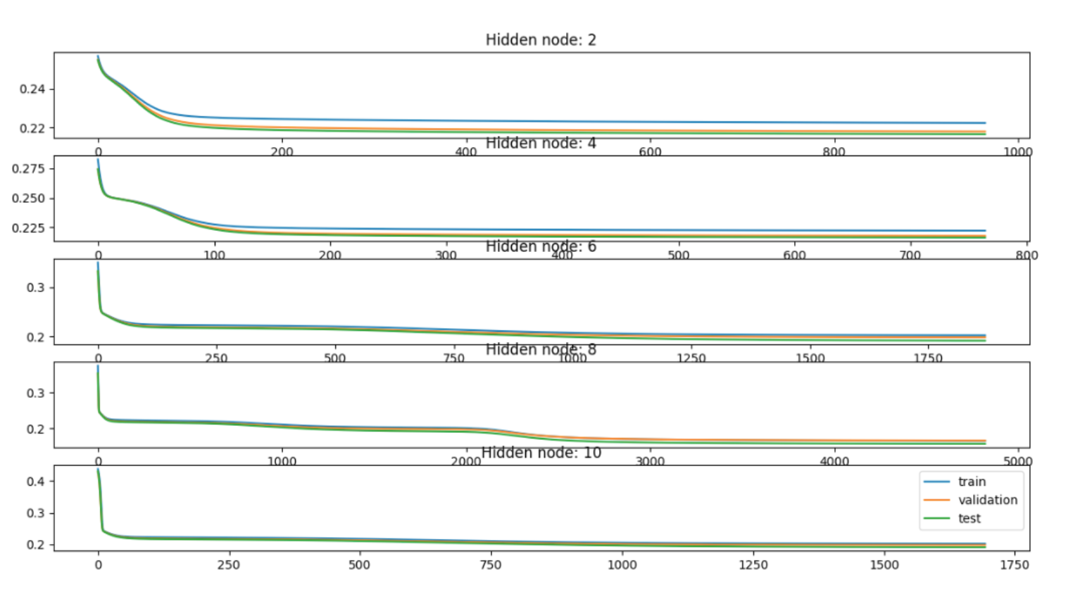
The below learning curves correspond to different number of hidden nodes (2,4,6,8 and 10).